Machine vision exposure time should be calculated from the object’s speed, the size of each pixel on the object and the amount of blur the inspection can tolerate. A shorter exposure limits movement within an image, while frame rate determines how often images are acquired. These settings solve different problems, and increasing frame rate alone does not guarantee a sharper image.
For a moving part, a practical starting point is to set a blur budget in pixels and calculate the longest exposure that stays within it. The remaining task is to collect enough light in that interval, synchronize the acquisition and confirm that the selected camera mode can sustain the required production rate.

Calculating Exposure Time from Motion
For approximately constant motion across the image plane, blur distance on the object equals speed multiplied by exposure time. Dividing that distance by the object-space pixel size expresses the blur in pixels. Rearranging the calculation gives the maximum exposure: allowable blur in pixels multiplied by object-space millimeters per pixel, divided by speed in millimeters per second.
Object-space pixel size follows from the field of view divided by the number of active pixels across that field. Use the image direction corresponding to the motion, and account for the actual magnification. The physical pixel pitch on a sensor is not the object-space pixel size unless the optical magnification is one-to-one.
There is no universal acceptable blur value for every inspection. An application detecting a large missing component may tolerate more blur than an application measuring a sharp edge or reading a fine marking. A half-pixel budget is a useful worked-example assumption, but the real limit should come from the measurement or detection requirement.
A Conveyor Example Using Iron 5514 BSI
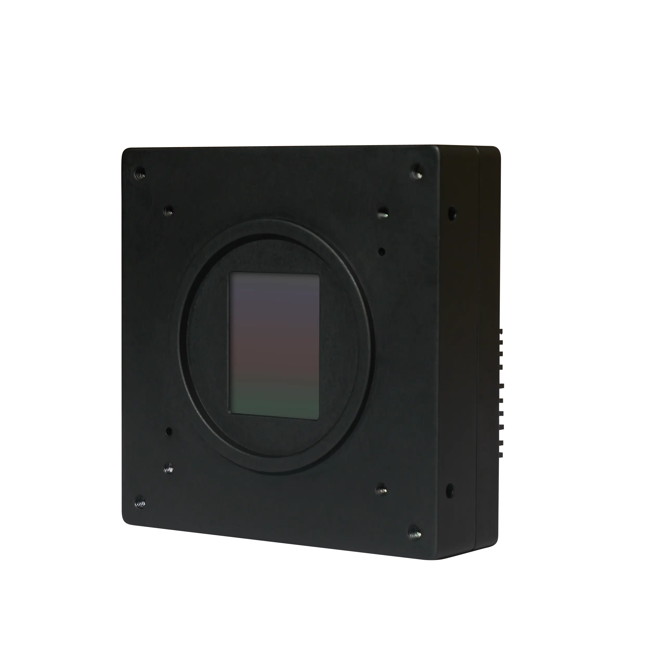
The Iron 5514 BSI has a 4,608 × 3,072 global-shutter sensor. Suppose a lens maps 180 mm across its 4,608-pixel dimension and the surface moves along that dimension at 2,000 mm/s. The object-space sampling is 180 / 4,608 = 0.03906 mm per pixel, approximately 39.1 µm.
For a half-pixel blur budget, the exposure limit is 0.5 × 0.03906 / 2,000 = 0.00000977 seconds, or approximately 9.8 µs. A 5 µs exposure corresponds to 0.26 pixel of travel; 10 µs corresponds to 0.51 pixel; 20 µs corresponds to 1.02 pixels. These calculated values describe motion during exposure, rather than measured image quality.
The camera lists a shortest exposure of 2.5 µs, so the example’s timing target is within its published exposure range. That does not establish adequate brightness at 5 or 9.8 µs. Lens transmission, illumination geometry, surface reflectance, wavelength and sensor response determine whether enough signal is available.
Why Frame Rate and Exposure Must Be Set Separately
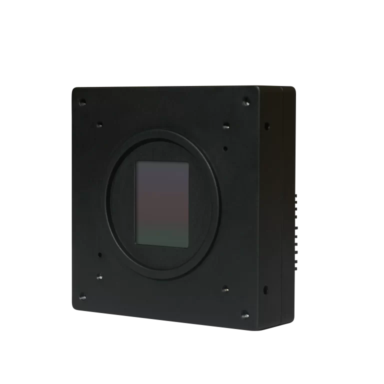
A camera operating at 200 frames/s begins successive frames 5 ms apart. It may expose each frame for only a small fraction of that interval. At 2,000 mm/s, the surface advances 10 mm between frame starts, while a 5 µs exposure records only 0.01 mm of travel. The first quantity controls temporal sampling and coverage; the second contributes to blur.
For continuous surface coverage, compare the distance traveled between frames with the usable field of view along motion. If the useful field is 120 mm and 10% overlap is required, successive frames can advance by 108 mm. At 2,000 mm/s the minimum coverage rate is approximately 18.5 frames/s. Tracking a fast event may require many more frames even when coverage alone is satisfied.
Readout constraints, exposure overlap and trigger modes affect which combinations are possible on a particular camera. Check the selected bit depth, region of interest and interface configuration. The line scan versus area scan comparison explains how coverage calculations change between the two architectures.
Global Shutter Prevents One Type of Distortion
A global shutter exposes the image array over a common interval. This is useful when the relative positions of features must represent the same moment. A rolling shutter starts and ends exposure at different times for different rows, so moving objects may appear skewed or distorted.
Neither shutter type makes exposure duration irrelevant. An object can still move several pixels during a long global-shutter exposure. Separating rolling-shutter distortion from ordinary motion blur avoids selecting a global-shutter camera and then expecting sharp images at any exposure setting.
Motion direction also matters. A rotating part has different image speeds at different radii, and camera vibration can move the whole image during an exposure. Use the fastest relevant feature motion when establishing the timing budget. The simple linear calculation is a first approximation when perspective or magnification changes substantially.
Using Strobe Lighting for Short Exposures
A short light pulse can define the effective illuminated exposure when ambient light contributes very little and the pulse falls inside the sensor’s exposure window. This can help deliver useful signal during a brief observation of a moving surface. If ambient illumination remains significant, the longer camera exposure may still record a blurred background around the strobed image.
Check the timing of the entire chain: trigger detection, camera delay, exposure start, light-controller delay and the actual optical pulse. The electrical command width is not always identical to the useful light-pulse width. Rise and fall times matter when the intended pulse lasts only a few microseconds.
Peak intensity, pulse duration and repetition rate must stay within the illumination system’s operating limits. A lighting setup that works for an occasional trigger may heat differently during continuous production. Validate contrast and timing at the highest expected trigger frequency, rather than only with isolated test images.
Choosing KAYA Cameras for Different Timing Priorities
The Iron 4502 is relevant when a process needs many observations per second and a 2,048 × 1,216 image provides enough spatial detail. Its current NS model specification lists up to 1,430 fps at 8 bits, 1,169 fps at 10 bits and 847 fps at 12 bits. The product page also lists external triggering and strobe-controller I/O. Its minimum exposure should be confirmed for the intended configuration, independently of those frame-rate figures.
Iron 5514 BSI provides a higher pixel count with published rates of 275 fps at 10 bits and 229 fps at 12 bits. This creates a different balance between the number of samples across a part and the number of observations over time. A 12-bit mode should be evaluated at its own achievable frame rate, rather than the 10-bit headline rate.
For a square field and fine spatial sampling, the Iron 0505 offers 5,120 × 5,120 pixels and a listed shortest exposure of 2.5 µs. Its High Speed version supports up to 150 fps at 8 bits and 145 fps at 10 bits; its Normal Speed version is specified at 41 fps at 8, 10 and 12 bits. The required image scale and observation rate determine which configuration is appropriate.
When Short Exposure Does Not Collect Enough Light
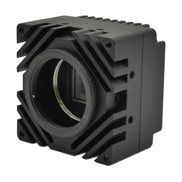
Once motion sets the exposure limit, increasing brightness by extending exposure may sacrifice the very detail the system needs to inspect. Evaluate illumination intensity and angle, lens aperture, optical transmission and spectral matching first. Opening the aperture also changes depth of field, so brighter images may come at the cost of focus tolerance.
Electronic gain changes the recorded signal level but does not collect additional photons. It may be useful within the camera’s noise and output-range constraints, yet it cannot replace the missing optical signal or recover clipped highlights. Judge the relevant feature’s contrast and repeatability, not just the overall brightness of the display.
For controlled scanning with repeated views of the same surface, digital TDI offers another approach: align several short observations and integrate their signals. It requires suitable acquisition and processing support. It does not reverse blur already present within each observation, and it should not be assumed to be a standard feature of every camera listed here.
Verifying the Exposure in the Actual Inspection
Start with representative good parts and the smallest relevant defects. Record the optics, field of view, speed, exposure, gain, light settings and camera mode. Compare edge detail and detection repeatability at the maximum process speed, including acceleration, vibration and variations in part height.
Check that triggers are accepted, images are transferred without loss and the decision is available when the machine needs it. If automatic exposure is used, constrain it so that it cannot exceed the established blur budget. A system that compensates for a darker part by extending exposure may quietly change the inspection quality.
Contact KAYA Vision with the speed range, field of view, target feature size and available illumination to review the camera configuration. Where the application requires motion-compensated integration or specialized timing, KAYA’s OEM camera development provides a route to evaluating those requirements together.